A visualization constructed using the vega-lite-api.

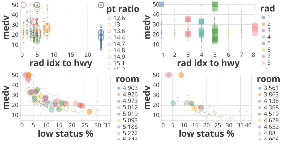
In this Boston Housing Dataset, the target variable is: medv, meaning the median value of owner-occupied homes. There is one field named rad, which is the index of accessibility to radial highways. The distribution of this variable is kind of interesting. For a group of houses, their values are the same as 24 (probably means hard to access to the highways). And for the rest houses data, the value ranges from 1 to 8. Therefore, it is naturally separate the datasets into two by this variable. I am wondering whether there is any difference between these two sub-datasets. The related 4 plots are explained below:

1. From the original data, the rad values distribution has a big separation, which naturally separate the dataset into two. So we save them as dataset01 and dataset02, respectively.
2. From dataset01, we visualized its relationship with medv in the 2nd plot (upper-right). The house price doesn't have any distictive pattern related to rad values (1-8).
3. Now to compare the medv and lstat relationship between dataset01 and dateset02, we plot 3rd and 4th ones accordingly, and use average room number per house (rm) in the color channel.
4. The lstat value distribution between these two datasets seems to be different. The lstat value concentrates higher value in dataset02 than in dataset01, which seems to indicate that the houses with rad as large as 24 will have more lower status population than the other dataset. Correspondingly, there are fewer high price houses, except a few of such exceptions which are close to Charles river, indicated by the big size of the circles.

See Data on Gist: Housing Values at Boston Suburbs

The original data comes from the github: Boston Housing Data